Timecourse of a Model: Autoplotting and saving as .jpeg
Johanna Daas
Setup
First, load the libraries needed for the workflow
library(tidyverse)
library(CoRC)
Input
Put in all variables needed to customise the workflow
Put in the path to the model (SBML), as url or local path (as string) and load the model. Use loadModel() for .cps models.
modelPathSBML <- "./Models/Schaber2012SUP_model.xml"
loadSBML(modelPathSBML)
#> # A COPASI model reference:
#> Model name: "Schaber2012SUP"
#> Number of compartments: 1
#> Number of species: 3
#> Number of reactions: 2
Set the timecourse settings. Further specifications are possible.
setTimeCourseSettings(duration  = 50,
                      intervals = 100)
Where should the .jpeg image be saved?
jpegPath <- "docs/timecourse.jpeg"Workflow
This should generally not need to be changed, only if the workflow is to be changed more generally.
# Check if path is already taken:
if(file.exists(jpegPath))
  stop("Error: This file does already exist.")
#> Error: Error: This file does already exist.

# Run time course
timecourse <- runTimeCourse()

# Autoplot time course
plot       <- autoplot.copasi_ts(timecourse)

# plot and save as pdf
jpeg(jpegPath)
print(plot)
dev.off()
#> quartz_off_screen
#>                 3
Output
This workflow produces the following output:
# Show the Plot
plot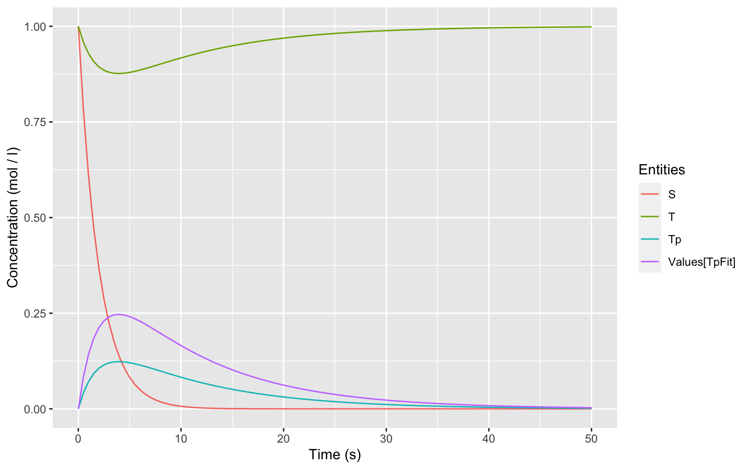
and saves the image in the file docs/timecourse.jpeg.